LaTeX guides
Maths to LaTeX: How to Convert Any Maths, With 150+ Examples
How to turn maths into LaTeX: write it yourself or convert handwriting, photos, PDFs, Word and AI output, with 150+ maths to LaTeX examples to copy.
Upload a photo or PDF of your notes and get a full LaTeX document back. For one equation, Text to LaTeX is free with no sign-up.
This is the quadratic formula in LaTeX:
x = \frac{-b \pm \sqrt{b^2 - 4ac}}{2a}Read it left to right and nearly every piece is a word. \frac takes a top and a bottom, each in braces. \pm is plus or minus. \sqrt puts a root over whatever is in its braces, and ^2 raises the 2. Converting maths to LaTeX is mostly that: a few dozen commands you use all the time, a handful of rules about braces and spacing, and a long tail of symbols you look up when you need them.
Below are the rules, more than 150 examples to copy, and the small details that decide whether your maths looks like a textbook or like a first attempt. After that come the routes for maths that starts somewhere other than your keyboard: handwritten notes, photos, PDFs, Word, maths software and AI chat.
Where is your maths now?
| Your maths is | The quickest way to LaTeX |
|---|---|
| In your head, or on the page in front of you | Type it, using the examples below |
| One symbol you cannot name | Draw it in a symbol finder |
| Handwritten, on paper or a tablet | A handwriting to LaTeX converter |
| A photo or a screenshot | A maths OCR tool |
| In a PDF | The original source if it exists, otherwise OCR |
| A Word or Google Docs equation | Word's LaTeX mode, or pandoc for a whole file |
| In Mathematica, Maple, MATLAB or Python | The software's own LaTeX export |
| A ChatGPT answer | Copy the code, then check it against the rendered maths |
How LaTeX writes maths
LaTeX does not read maths from a picture. You describe it in plain text and LaTeX does the layout. Six rules get you a long way.
- Maths goes in maths mode. In a sentence, that means single dollar signs:
$x^2 + 1$gives . An equation on its own line goes in\[ ... \]. Outside maths mode,x^2is an error, and LaTeX tells you so with "Missing $ inserted" (how to read that). ^and_apply to one character. Anything longer needs braces:x^{10}gives , whilex^10gives , and compiles without a word of complaint.- Commands start with a backslash:
\alpha,\times,\infty,\sin. Forgetting the backslash on a function name is the most common mistake in student LaTeX, becausesin xis set as the variables , and multiplied by . - Braces group things and do not print.
\frac{a+b}{2}and\sqrt{x+1}use them to say what belongs together. To print a brace, write\{or\}. - Spaces you type in maths are ignored. LaTeX spaces maths by what each symbol is, so a relation like gets more room than an operator like , and
a=bcomes out the same asa = b. To add space yourself, use\,for a thin gap or\quadfor a wide one. The spacing guide has the full set. - Words go in
\text{}.\text{if } x > 0keeps the word upright with its space. Without it, LaTeX reads "if" as times .
Here is a sentence of maths written with those rules, "the derivative of x squared sin x is 2x sin x plus x squared cos x":
\[ \frac{d}{dx}(x^2 \sin x) = 2x \sin x + x^2 \cos x \]Nearly everything on this page works in a bare LaTeX document. A few commands come from packages: amsmath gives you align, cases, the matrix environments, \text and \binom; amssymb gives you \mathbb and \varnothing; mathtools gives you \coloneqq. The document at the end loads all three.
Maths to LaTeX: examples to copy
The left column is the maths as it looks on a line of its own, the right column is what to type. Put the code inside $...$ in a sentence or \[ ... \] on its own line.
Fractions, powers and roots
| Maths | LaTeX |
|---|---|
\frac{a}{b} | |
\tfrac{1}{2}, a small fraction for a line of text | |
\dfrac{1}{2}, full size even in a line of text (it pushes the lines apart, see below) | |
\frac{1}{1 + \frac{1}{x}} | |
\cfrac{1}{1 + \cfrac{1}{1 + x}}, a continued fraction that stays full size as it nests | |
x^2 | |
x^{n+1} | |
x_1 | |
x_{ij} | |
x_1^2 | |
e^{-x^2} | |
x^{-1/2} | |
10^{-3} | |
\sqrt{x} | |
\sqrt[3]{x} | |
\sqrt{b^2 - 4ac} |
More in the guides to fractions and square roots.
Greek letters
| Maths | LaTeX |
|---|---|
\alpha | |
\beta | |
| , | \gamma, \Gamma |
| , | \delta, \Delta |
| , | \varepsilon, \epsilon (the first is the one most people write by hand) |
| , , | \theta, \vartheta, \Theta |
| , | \lambda, \Lambda |
\mu | |
\nu | |
| , | \pi, \Pi |
\rho | |
| , | \sigma, \Sigma |
\tau | |
| , , | \varphi, \phi, \Phi (again, the first is the handwritten shape) |
\chi | |
| , | \psi, \Psi |
| , | \omega, \Omega |
Capital Greek letters that look like Latin ones have no command: a capital alpha is just A, a capital rho is P. There is no \omicron either; it is an o. The whole alphabet is in the Greek letters guide.
Operators and relations
| Maths | LaTeX |
|---|---|
a \times b | |
a \cdot b | |
a \div b | |
| , | \pm, \mp |
a \neq b | |
| , | a \leq b, a \geq b |
a \approx b | |
a \equiv b \pmod{n} | |
y \propto x | |
a \sim b | |
| , | a \ll b, a \gg b |
x \to \infty | |
x \mapsto x^2 | |
f \circ g | |
a \coloneqq b, "is defined as" (needs mathtools) |
See the times, plus or minus, less than or equal to and proportional to guides.
Brackets and bars
| Maths | LaTeX |
|---|---|
\left( \frac{a}{b} \right)^2 | |
\bigl( a + b \bigr), a fixed size up from normal | |
\{ 1, 2, 3 \} | |
\lvert x \rvert | |
\lVert \mathbf{v} \rVert | |
| , | \lfloor x \rfloor, \lceil x \rceil |
\langle u, v \rangle | |
\left. \frac{dy}{dx} \right\rvert_{x=0}, evaluated at a point |
\left. is an invisible bracket, there because every \left needs a partner. More in the guides to brackets and absolute values.
Functions, logs and trigonometry
| Maths | LaTeX |
|---|---|
| , , | \sin x, \cos x, \tan x |
| , , | \sec x, \csc x, \cot x |
\cos^2 \theta | |
\tan^{-1} x | |
\arcsin x | |
\sinh x | |
\ln x | |
\log_{10} n | |
\exp(x) | |
\gcd(a, b) | |
f\colon A \to B | |
\max_{x \in S} f(x) | |
\operatorname{sgn}(x) | |
\operatorname*{arg\,max}_{x} f(x) |
\operatorname{} sets any name upright like the built-in functions, and the starred form puts limits underneath in display maths. See the trigonometric functions and logarithms guides.
Calculus
| Maths | LaTeX |
|---|---|
\lim_{x \to 0} \frac{\sin x}{x} = 1 | |
\lim_{h \to 0} \frac{f(x+h) - f(x)}{h} | |
\lim_{n \to \infty} a_n | |
\frac{dy}{dx} | |
\frac{d^2 y}{dx^2} | |
| , | f'(x), f''(x) |
| , | \dot{x}, \ddot{x} |
\frac{\partial f}{\partial x} | |
\frac{\partial^2 f}{\partial x \, \partial y} | |
\nabla f | |
| , | \nabla \cdot \mathbf{F}, \nabla \times \mathbf{F} |
\int f(x)\,dx | |
\int f(x)\,\mathrm{d}x, with an upright d | |
\int_a^b f(x)\,dx | |
\int_0^\infty e^{-x}\,dx = 1 | |
\Bigl[ F(x) \Bigr]_a^b | |
\iint_D f\,dA | |
\oint_C \mathbf{F} \cdot d\mathbf{r} |
More in the guides to derivatives, integrals and the partial derivative symbol.
Sums, products and series
| Maths | LaTeX |
|---|---|
\sum_{i=1}^{n} i | |
\sum_{n=0}^{\infty} \frac{x^n}{n!} | |
\sum_{\substack{1 \le i \le n \\ i \text{ odd}}} a_i, two lines of conditions | |
\prod_{k=1}^{n} k | |
n! | |
\binom{n}{k} | |
a_1 + a_2 + \dots + a_n | |
a_1, a_2, \dots, a_n | |
\sum_{i,j} a_{ij} |
In a line of text the limits of a sum sit beside it; on a line of its own they go above and below. See the sum and product guides and binomial coefficients.
Vectors and matrices
| Maths | LaTeX |
|---|---|
\vec{v} | |
\mathbf{v} | |
\boldsymbol{\mu}, for bold Greek letters | |
| , | \hat{\imath}, \hat{\jmath}, with the dots removed |
\overrightarrow{AB} | |
\mathbf{u} \cdot \mathbf{v} | |
\mathbf{u} \times \mathbf{v} | |
\begin{pmatrix} a & b \\ c & d \end{pmatrix} | |
\begin{bmatrix} 1 & 0 \\ 0 & 1 \end{bmatrix} | |
\begin{Bmatrix} a & b \\ c & d \end{Bmatrix} | |
\begin{vmatrix} a & b \\ c & d \end{vmatrix}, a determinant | |
\begin{Vmatrix} a & b \\ c & d \end{Vmatrix} | |
\begin{pmatrix} x \\ y \\ z \end{pmatrix} | |
\begin{pmatrix} a_{11} & \cdots & a_{1n} \\ \vdots & \ddots & \vdots \\ a_{m1} & \cdots & a_{mn} \end{pmatrix} | |
A^{\mathsf{T}} | |
A^{-1} | |
\det(A) | |
\operatorname{tr}(A) |
& separates columns and \\ ends a row, and the environment chooses the brackets. An augmented matrix, for row reduction, is an array with a | in its list of columns:
\left[ \begin{array}{cc|c} 1 & 2 & 5 \\ 3 & 4 & 6 \end{array} \right]More in the matrices and vectors guides.
Sets and logic
| Maths | LaTeX |
|---|---|
| , | x \in A, x \notin A |
| , | A \subseteq B, A \subset B |
| , | A \cup B, A \cap B |
A \setminus B | |
| , | A^c, \overline{A} |
A \times B | |
| , | \varnothing, \emptyset |
| , , , , | \mathbb{R}, \mathbb{N}, \mathbb{Z}, \mathbb{Q}, \mathbb{C} |
\mathbb{R}^n | |
\{ x \in \mathbb{R} \mid x > 0 \} | |
| , | \forall x, \exists x |
\exists!\, x | |
| , | p \implies q, p \iff q |
\neg p | |
| , | p \land q, p \lor q |
| , | \therefore, \because |
See the guides to element of, union, intersection, the empty set, real numbers, for all and implies.
Probability and statistics
| Maths | LaTeX |
|---|---|
P(A \mid B) | |
P(A \cup B) = P(A) + P(B) - P(A \cap B) | |
\mathbb{E}[X] | |
\operatorname{Var}(X) | |
\operatorname{Cov}(X, Y) | |
\bar{x} | |
\hat{\theta} | |
X \sim \mathcal{N}(\mu, \sigma^2) | |
\binom{n}{k} p^k (1-p)^{n-k} | |
s = \sqrt{\frac{1}{n-1} \sum_{i=1}^{n} (x_i - \bar{x})^2} |
Geometry
| Maths | LaTeX |
|---|---|
90^\circ | |
\angle ABC | |
\triangle ABC | |
\overline{AB} | |
AB \parallel CD | |
AB \perp CD | |
\triangle ABC \cong \triangle DEF | |
\triangle ABC \sim \triangle DEF |
See the degree, angle, parallel and perpendicular guides.
Physics and units
| Maths | LaTeX |
|---|---|
\mathbf{F} = m\mathbf{a} | |
E = h\nu | |
\hbar | |
\Delta x \, \Delta p \geq \frac{\hbar}{2} | |
\langle \psi \vert \phi \rangle | |
g = 9.81\,\mathrm{m\,s^{-2}} | |
25\,^\circ\mathrm{C} |
Units are set upright with a thin space after the number. If you write a lot of them, the siunitx package does it for you: \qty{9.81}{\metre\per\second\squared}.
Details that make LaTeX maths look right
Everything in this section compiles either way. LaTeX will not warn you, and the difference only shows on the page, which is why these are the things that separate maths that looks typeset from maths that looks typed. Each pair below was typeset by pdflatex.
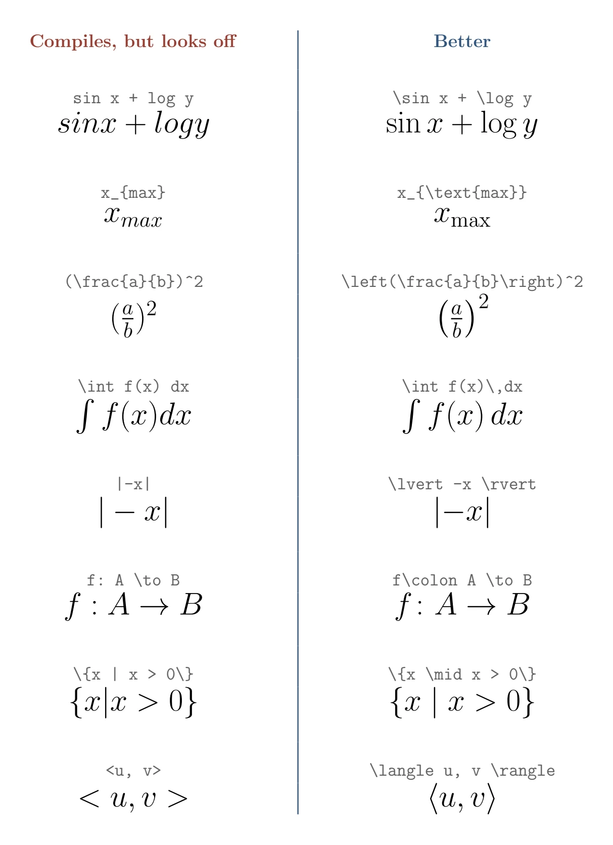
- Function names need their backslash.
\sin,\log,\max,\detand the rest are set upright, as names. For one LaTeX does not know, use\operatorname{sgn}, or put\DeclareMathOperator{\sgn}{sgn}in the preamble once and write\sgn xfrom then on. - A subscript that is a word or a label, like max or eff, should be upright:
x_{\text{max}}. A subscript that is a variable, like the in , stays italic. Inside a theorem, where the text is italic,\textturns italic with it, so\mathrm{max}is the safer choice there. More in text in maths mode. \left(and\right)make brackets grow to fit what is inside. Use them around tall things such as fractions and sums, not everywhere: around a plainxthey change nothing except to add a gap after a function name (\sin\left(x\right)), and a\leftcannot be split from its\rightacross the lines of analign. For a fixed size, use\bigl(and\bigr), or\Bigl(and\Bigr)for larger.\,before thedxgives the thin space printed books use. Some styles also set the d upright,\mathrm{d}x, as the ISO 80000-2 standard recommends; most English textbooks keep it italic. Either is fine if you are consistent.- A plain
|is an ordinary symbol, so in|-x|LaTeX reads the minus as a subtraction and spaces it.\lvertand\rvertmark the bars as opening and closing, and the minus sits tight. Norms work the same way with\lVertand\rVert. - A plain colon is a relation, like an equals sign, so
f: A \to Bgets equal space either side of it.\colonis the punctuation colon used in function notation. \midis the bar in set-builder notation and in , with space on both sides. A typed|gets none. See the mid symbol guide.<and>are less than and greater than. Angle brackets are\langleand\rangle.
A few more that do not show in the picture:
\varepsilonand\varphiare the shapes most people write by hand;\epsilon() and\phi() are the alternatives. Pick one of each and use it throughout. See epsilon and phi.- With
amsmath,\dotschooses its own height from what follows it: centred ina_1 + \dots + a_n, on the line ina_1, \dots, a_n. To choose yourself, use\cdotsor\ldots, and\vdotsand\ddotsin matrices. See the dots guide. \mathbf{\mu}leaves a lowercase Greek letter as it was. Bold Greek needs\boldsymbol{\mu}, or\bmfrom thebmpackage. See bold and italic maths.:=sits its colon slightly low against the equals sign.\coloneqqfrommathtoolscentres it.
Layouts: cases, working and numbered equations
Some maths is as much layout as symbols. These need an environment from amsmath, so they go on lines of their own.
A function defined in pieces uses cases. Each line is the value, then &, then the condition:
\[
  \lvert x \rvert =
  \begin{cases}
    x  & \text{if } x \geq 0, \\
    -x & \text{if } x < 0.
  \end{cases}
\]Working over several lines uses align*, with & just before each equals sign so the signs line up:
\begin{align*}
  (x + 2)^2 &= (x + 2)(x + 2) \\
            &= x^2 + 2x + 2x + 4 \\
            &= x^2 + 4x + 4
\end{align*}Without the star, align numbers every line. If an old template or an AI answer gives you eqnarray instead, change it to align: eqnarray puts too much space around the equals signs, and l2tabu, the standard list of obsolete LaTeX, has warned against it for years.
An equation you want to refer back to goes in equation with a label. LaTeX numbers it and fills in the number wherever you write \eqref, so the references stay right when you add equations above it:
\begin{equation}
  e^{i\pi} + 1 = 0
  \label{eq:euler}
\end{equation}
Equation \eqref{eq:euler} links five constants.
Three more that come up often. A brace under part of an expression, , is \underbrace{1 + 1 + \dots + 1}_{n \text{ times}} (see overbrace and underbrace). A symbol written over another, , is \overset{\text{def}}{=}. A box round a final answer, , is \boxed{x = 3}. Simultaneous equations have their own guide.
Handwritten maths to LaTeX
Retyping handwritten working is where most of the time goes, and where mistakes creep in: a minus sign dropped on line four survives all the way to the final answer. A converter does the typing, and your job becomes checking.
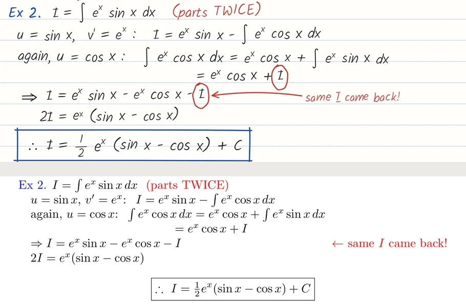
For whole pages, a handwriting to LaTeX converter reads a photo or PDF of your notes and gives back one LaTeX document, with fractions, matrices and lines of working in shape. LatexNotes does this for full lecture notes and redraws hand-drawn graphs as TikZ code you can edit. On an iPad you can also write straight into a LatexNotes notebook with an Apple Pencil and convert any part of the page in place. Notes already in Goodnotes have their own route.
For a single equation inside Goodnotes, its own Math Conversion works: lasso the equation, choose Convert and then Math, and copy or share the result as LaTeX.
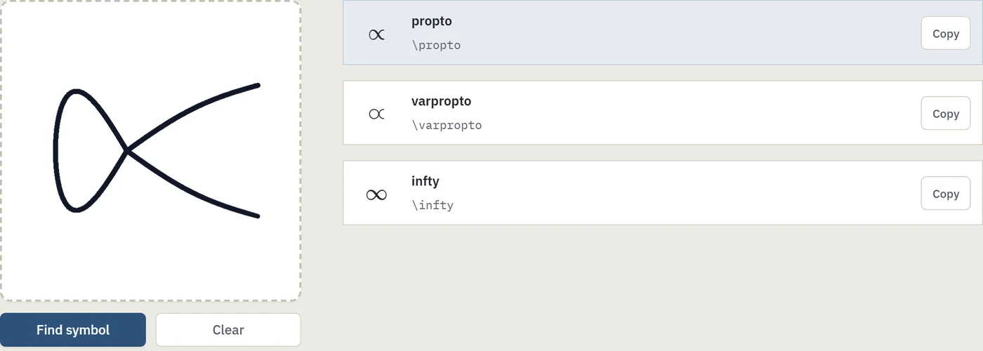
For one symbol whose name you do not know, draw it. The LatexNotes symbol finder and Detexify both name a symbol from a rough sketch.
What trips up a converter is what trips up anyone reading your notes: a that could be an , a that could be a , a that could be an or a bar, a superscript that touches the line above it, a scribble over a mistake. Dark ink, a little space between lines and one clean line through crossed-out work fix most of it. And read the typeset result against the page before you hand it in. A misread symbol usually still compiles, so nothing else will catch it.
A photo or screenshot of maths
A photo of a whiteboard, a textbook page or a screenshot of a lecture slide goes through photo to LaTeX or any other maths OCR tool (OCR, optical character recognition, is software that reads text from an image). Printed maths converts far more reliably than handwriting. Crop to the maths you want, so nothing nearby gets read as part of it. Shoot straight on rather than at an angle, which squashes fraction bars and subscripts. And if the maths is on a screen, take a screenshot rather than a photo of the screen. Maths OCR explains how the recognition works and where it struggles.
Maths in a PDF
Copying maths out of a PDF almost never works. A PDF records which character goes where on the page, not the LaTeX that put it there, so a pasted integral arrives as a scatter of symbols and numbers.
If the PDF is a paper on arXiv, get the authors' own LaTeX instead: the TeX Source link on the paper's abstract page downloads it. Lecturers will often share their source if you ask. Otherwise, convert the page as an image. PDF to LaTeX reads typed and handwritten PDFs page by page and gives back one document.
Word and Google Docs equations
Word for Microsoft 365 can show any equation as LaTeX:
- Click into the equation.
- On the Equation tab, choose LaTeX as the input format.
- Press Ctrl + Shift + = to switch the equation to linear format. It now reads as LaTeX code you can copy.
- Press Ctrl + = to turn it back.
If LaTeX is not on your Equation tab, your version of Word only has UnicodeMath, which looks similar but is not LaTeX.
For a whole Word document, the free command-line tool pandoc converts a .docx file to LaTeX, equations included:
pandoc notes.docx -o notes.texComplicated layouts can need tidying afterwards, but it beats retyping a document.
Google Docs cannot export its equations as LaTeX. Take a screenshot and convert it as a photo, or retype it with the examples above. Its equation editor does accept LaTeX-style shortcuts such as \alpha and \frac, so typing them will already feel familiar.
Markdown, Obsidian and Notion
If your notes are in Markdown, the maths is probably LaTeX already. Obsidian and most Markdown editors put maths between dollar signs, $...$ in a line and $$...$$ on its own line, using LaTeX commands. Notion's equations are LaTeX too; click one to see its code. You can copy the maths across as it is. The one change for a LaTeX document is to swap $$...$$ for \[ ... \], for the reason below.
LaTeX from maths software
Computer algebra systems write their results as LaTeX directly, which saves copying a long expression by hand.
| Software | How to get LaTeX |
|---|---|
| Mathematica | TeXForm[expr] |
| Maple | latex(expr) |
| MATLAB (Symbolic Math Toolbox) | latex(S) for a symbolic expression S |
| Python with SymPy | latex(expr) |
The output is correct but written for a machine. Here is SymPy integrating :
from sympy import symbols, integrate, sin, latex

x = symbols("x")
print(latex(integrate(x**2 * sin(x), x)))- x^{2} \cos{\left(x \right)} + 2 x \sin{\left(x \right)} + 2 \cos{\left(x \right)}Every function argument is wrapped in \left( and \right), and every power gets braces it does not need. It compiles, but it reads badly as source and the brackets add nothing. SymPy's fold_func_brackets=True option drops them, giving - x^{2} \cos {x} + 2 x \sin {x} + 2 \cos {x}, and a minute of tidying by hand gets you what you would have written yourself:
-x^2 \cos x + 2x \sin x + 2 \cos xChatGPT and other AI
Chatbots are good at LaTeX syntax. Where they go wrong is the maths. Asked to convert, they sometimes simplify, reorder or quietly correct it, and a changed sign or index looks perfectly reasonable in code. A few habits keep that from reaching your work:
- Say exactly what you want: "Convert this to LaTeX exactly as written, without simplifying. Use amsmath, put the working in align*, and return only the code."
- Render the answer and compare it with the original symbol by symbol. Reading the code is not enough.
- Watch for things that work in a chat window but not in a LaTeX document. Pasted symbols such as π or ≤ stop pdflatex with "Unicode character not set up for use with LaTeX".
$$...$$andeqnarraywork but are best replaced. Old plain TeX such as{a \over b}makesamsmathwarn "Foreign command \over". - For a page of notes rather than one equation, use a converter built for documents. A chat answer tends to summarise or skip, where a converter keeps every line.
If you would rather describe maths in words than type commands, Text to LaTeX turns a description such as "integral from 0 to pi of sine x" into LaTeX, with a preview.
Reading LaTeX errors
Converted LaTeX is usually right, and when it is not, the error message says where. Here is what pdflatex printed for a sentence with a power typed outside maths mode:
! Missing $ inserted.
<inserted text>
                $
l.4 The side is 3 metres, so the area is 3^
                                           2 = 9 square metres.
Every TeX error has this shape. The line starting with ! says what went wrong. The line starting l.4 is line 4 of your file, broken at the point where TeX gave up: just after the ^, which only means something in maths mode. TeX then reported a second "Missing $" on line 5, which was only a knock-on of the first, so always fix the first error and compile again before reading the rest.
An "Undefined control sequence" points at the command it does not know in the same way. Here it is \mathbb, used without \usepackage{amssymb}:
! Undefined control sequence.
l.4 Let $f\colon \mathbb
                        {R} \to \mathbb{R}$ be continuous.
The ones you will meet most:
| Error message | Usual cause | Fix |
|---|---|---|
| Missing $ inserted | A maths command such as x^2 or \alpha outside maths mode | Put the maths in $...$ |
| Undefined control sequence | A misspelt command, or one from a package that is not loaded | Check the spelling, or load amsmath or amssymb |
| Missing \right. inserted | A \left with no matching \right | Add the \right) it needs, or \right. for no bracket |
| Extra }, or forgotten $ | Unbalanced braces | Count the braces in the equation |
| Misplaced alignment tab character & | An & outside align, cases or a matrix | Put the lines in an environment |
| Unicode character not set up for use with LaTeX | A pasted symbol such as π or ≤ | Replace it with \pi or \leq |
To test one equation without setting up a document, paste it into the LaTeX equation editor and check the preview.
Inline or display maths, and a document that compiles
Maths inside a sentence goes in $...$, or the equivalent \( ... \). Maths on its own line goes in \[ ... \], or in equation if you want it numbered. The difference is more than position: inline maths is squeezed to fit the height of the line, and display maths gets full size.
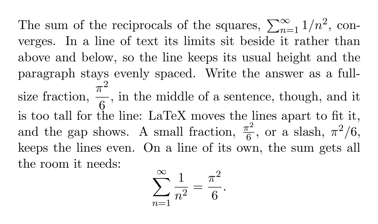
You will see $$...$$ used for display maths in Markdown and all over the web. It usually works in LaTeX too, but it is plain TeX rather than LaTeX: it ignores the fleqn option that sets equations flush left and can leave uneven space above an equation. In a LaTeX document, \[ ... \] is the right choice.
This document loads the three packages the examples on this page use. Paste any of them between \begin{document} and \end{document} and it will compile:
\documentclass{article}
\usepackage{amsmath, amssymb, mathtools}

\begin{document}

The roots of $ax^2 + bx + c = 0$ are
\[
  x = \frac{-b \pm \sqrt{b^2 - 4ac}}{2a}.
\]

\end{document}
Open it in LatexNotes, Overleaf or any LaTeX editor. For whole documents rather than single equations, the LaTeX templates are set up for notes, homework and reports, and the LaTeX symbols list has every symbol on one page.
Frequently asked questions
How do I convert maths to LaTeX?
Write it in maths mode with LaTeX commands, such as \frac{a}{b} for a fraction and x^2 for a power, or use a converter: a maths OCR tool for handwriting, photos and PDFs, Word's LaTeX mode for Word equations, or the LaTeX export in software such as Mathematica or SymPy.
Is there a free maths to LaTeX converter?
Yes. LatexNotes' Text to LaTeX is free with no sign-up: type or describe an equation and copy the LaTeX. The LatexNotes symbol finder names any symbol you draw. Converting pages of handwritten notes needs a free account.
Can I convert handwritten maths to LaTeX?
Yes. Photograph or scan the page, or write on a tablet, and use a handwriting to LaTeX converter. Dark ink, space between lines and clearly different look-alike symbols (an x and a times sign, a v and a nu) make the result much more accurate. Check the typeset result against the page, because a misread symbol usually still compiles.
Why does my LaTeX maths compile but look wrong?
Usually a missing backslash on a function name (sin x instead of \sin x), a word typed straight into maths instead of \text{}, brackets that do not grow round a fraction (use \left( and \right)), or a typed | or < where \mid, \lvert or \langle was meant.
How do I get LaTeX from a Word equation?
In Word for Microsoft 365, click into the equation, choose LaTeX as the input format on the Equation tab, then press Ctrl + Shift + = to show the equation in linear format, which is its LaTeX code. For a whole document, pandoc converts a .docx file to LaTeX, equations included.
Can ChatGPT convert maths to LaTeX?
Yes, for single equations and short derivations, but it can change the maths while converting it. Always render the code and compare it with the original before you use it.
What is the difference between inline and display maths in LaTeX?
Inline maths, written between single dollar signs, sits inside a line of text. Display maths, written in \[ ... \], goes on its own line, centred and full size. Use the equation environment instead when you want the equation numbered.
Why does LaTeX say "Missing $ inserted"?
A maths command such as x^2 or \alpha is outside maths mode. Put the maths between dollar signs, or inside \[ ... \] on its own line.
Sources
- Microsoft Support, Linear format equations using UnicodeMath and LaTeX in Word.
- John MacFarlane, Pandoc User's Guide, and its maths converter texmath.
- American Mathematical Society, amsmath, the package behind
align,casesand the matrix environments. - Morten Høgholm and others, mathtools, for
\coloneqq. - Mark Trettin, l2tabu: an annotated list of obsolete LaTeX commands and packages, on
$$andeqnarray. - Joseph Wright, siunitx, for typesetting units.
- ISO 80000-2:2019, Quantities and units, Part 2: Mathematics, which sets the differential d upright.
- Wolfram Language documentation, TeXForm.
- MathWorks, latex: LaTeX form of a symbolic expression.
- SymPy documentation, Printing.
- Daniel Kirsch, Detexify, LaTeX symbol recognition from a drawing.